Linear Interpolation: Online Calculator + Excel & Manual Method

Linear interpolation is a simple yet powerful mathematical technique used to estimate an unknown value between two known data points that are linearly connected. In other words, if you know the values of two points on a straight line, you can calculate the value of any point that lies between them.

In this article, we will explore three different ways to perform linear interpolation, starting with the most convenient:

Online Calculator – instantly computes results and shows step-by-step working.
Excel TREND Function – a built-in feature to perform interpolation in spreadsheets.
Manual Calculation – applying the standard formula to verify results step by step.

By learning all three methods, you can quickly solve interpolation problems and cross-check your answers with confidence.

Table of Contents

Linear Interpolation via Online Calculator

x₁: y₁: x₂: y₂: Find y at x:

Linear Interpolation Through Excel function (Trend)

Data

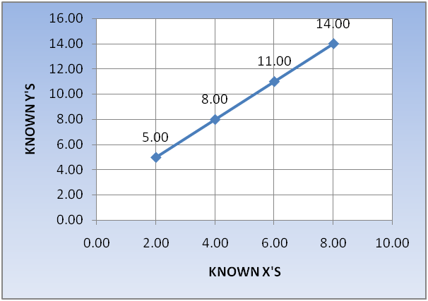
Take the following data and calculate Y corresponds to X = 5:

Known X’s	Known Y’s
2.00	5.00
4.00	8.00
6.00	11.00
8.00	14.00

Table 1:Available Data

Required

To calculate the value of Y corresponds to X = 5

Condition

Points are linearly connected. we know that it means if we draw the lines then lines has constant slope

Procedure

Select the output cell, then click on Insert function “fx”
In the search bar type “Trend” and click on Go

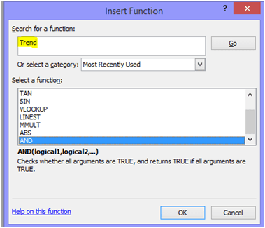
Select “Trend” and press OK

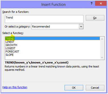
Below Window appears on the screen

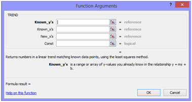
In the Known Y’s range select your Y range values, In the X’s range select the corresponding X range values. Here New X’s is the value, for which the corresponding Y is required. “Const” is an optional argument it will be “True” or an empty cell, if there is Y-intercept, it will be false if we know the constant term is 0.

Apply formula for the given data as shown in the below picture:

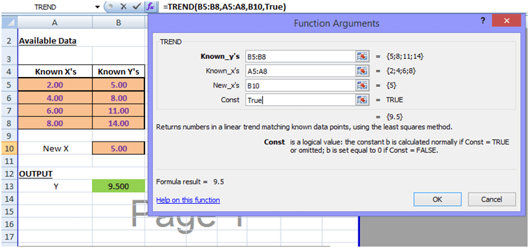
Press OK, in the output cell you get value of Y=9.5 corresponding to the X=5

Attachment

I am attaching an Excel sheet of linear interpolation, which makes your calculation easier and faster;

Linear-Interpolation Download

Manual Linear Interpolation Step by Step

Here we calculate “Y” at the corresponding new value X = 5 and verify the output result of the Excel function “Trend”

First, select the two points X1 & X2 and take corresponding Y’s values (i.e. Y₁ & Y₂)

Take;

X₁=4.0 and corresponding Y₁=8.0

X₂=6.0 and corresponding Y₂=11.0

Since points are linearly connected means having a constant slope (m₁=m₂), therefore,

Since the manually calculated value is the same as the value calculated from the “Trend function” of Excel, therefore, result is verified.

Conclusion

In this article, we explored three practical ways to perform linear interpolation: using an online calculator, the Excel TREND function, and manual calculation.

The calculator offers instant results with step-by-step working, making it the fastest way to verify values.
The Excel TREND function is efficient when handling large datasets, allowing you to interpolate thousands of values in just a few clicks.
The manual method helps you understand the underlying formula and ensures you can cross-check results independently.